What this article is about is an explanation of the basic methods used in JoBS to answer questions about basketball. In order to determine how controlling tempo, for instance, can help win games, you need a measurement of tempo. You also need to know what wins games. What follows is the framework used in JoBS to answer this sort of question.
Basketball teams constantly exchange possession of the basketball. When a team makes a shot, their opponents get the ball by rule. When a team misses a shot and their opponents rebound, possessions alternate. When there is a turnover, that is, by definition, a change of possession. This is all obvious, you scientifically critical readers should be thinking, but what about when a team misses a shot and gets their own rebound? Is this two possessions in a row for the same team?
Not in JoBS, it isn't. People have defined possessions this way, including the late great college coach, Frank McGuire, in his book, Defensive Basketball. Was he wrong? There is no right or wrong here, just more useful and less useful. If one defines a sequence with an offensive rebound as one continuous possession, rather than two in a row, you have a very solid framework for analyzing teams and players. It yields the statement made at the start of this section: opposing teams have the same number of possessions with which to score in a game. If you don't define them this way, you cannot make this statement.
A consequence of this tenet is that points per possession (or points per 100 possessions, as I like to use) is a consistent way of evaluating offenses and defenses. It does this by removing the pace of the game from a measurement of offense or defense. Points per game is "contaminated" by teams that slow the game or push the pace so much that the efficiency with which they score is hidden by that pace. By removing pace, we evaluate how efficiently a team scores points through shooting, passing, picking, and offensive rebounding. This last one is critical. By defining possessions this way, offensive rebounds are seen as, well, an offensive contribution. Rather than classifying things as offense, defense, or rebounding, the offensive rebounds are categorized with the offense and the defensive rebounds are categorized with the defense. At the NBA level, this is mostly a question of pedantics, but basketball can be and is taught this way -- where offensive rebounds are a part of the offense. When you are coaching a team, you give them all the tools necessary for how to score and, at the lower levels, in particular, where shooting percentages are not that high, the better offenses are determined by how well they get offensive rebounds.
If you would like to read more about possessions and how they were developed for use in this journal, see Introduction to Methods, New Measurement Techniques and A Binomial Model of the Game of Basketball, or Established Methods, my summary of the techniques used here.
Floor percentage is an obvious concept for teams. It is less obvious for individuals, but it can still be defined, as will be discussed in a later section.
Since teams and their opponents have the same number of possessions in a game and, hence, in a season (for example, Kentucky's offense has 3000 possessions in a season and their opponents also have 3000 possessions in a season), offensive ratings and defensive ratings have the same relationship as points per game scored and allowed. A team that outscores their opponents per game also outscores their opponents per possession. In fact, there is a fairly predictable relationship between points scored vs. points allowed and winning percentage. That relationship is the same between offensive rating vs defensive rating and winning percentage ...
                            (Points Scored)^16.5
Expected Win% = --------------------------------------------
                (Points Scored)^16.5 + (Points Allowed)^16.5
This formula comes from the analogous one from baseball (which
has an exponent of 2, not 16.5), which got its name from a
similar looking formula from high school trigonometry. Basically,
the formula translates a points per game (or just points) differential
into an expected winning percentage. One of its principal advantages
is that it also applies to the offensive and defensive ratings presented
in the previous section:
                             (Offensive Rating)^16.5
Expected Win% = -------------------------------------------------
                (Offensive Rating)^16.5 + (Defensive Rating)^16.5
This equation gives the exact same result as
the previous one for a given team. This implies that
if offensive and defensive ratings can be obtained for
individual players (which they can), this equation can be used
to determine a winning percentage for players.
This is the bottom line -- increasing winning percentage. Having a good translation between winning percentage and all other methods is then vital for any of these methods to succeed. The Pythagorean Method is quite good for teams, having a 95% correlation with actual wins. A second method that estimates winning percentage based on points scored and allowed is the Correlated Gaussian method. This method has several advantages over the Pythagorean method, including accuracy, being correlated with wins slightly better. This method was derived from a theory laid out in two reports ( Basketball's Bell Curve and New Measurement Techniques and A Binomial Model of the Game of Basketball). I will not present the theory here, but the theory makes this method much more powerful than the Pythagorean alternative. It also makes the formula more complicated:
                     __                                                    __
                     |               (PPG-PPG Allowed)                      |
Expected Win% = NORM |------------------------------------------------------|
                     |SQRT[Var(PPG)+Var(PPG Allowed)-2*Cov(PPG,PPG Allowed)]|
                     --                                                    --
where
PPG			Average points scored per game
PPG Allowed		Average points allowed per game
SQRT[]			Square root of the quantity in brackets []
Var(PPG)		Statistical variance of PPG
Var(PPG Allowed)	Statistical variance of PPG allowed
Cov(PPG,PPG Allowed)	Statistical covariance between PPG and PPG allowed
NORM[]			A function to find the probability that a random
			draw from a Gaussian distribution with an
			average of zero and a variance of one is less than
			the quantity in brackets []
I apologize to those not familiar with college level statistics. Heck, I apologize to those familiar with college level statistics enough that they wanted to forget them. But this method is necessary and the concept is not as difficult as the terminology makes it out to be. I will demonstrate what this means below or you can read the article on Basketball's Bell Curve, which talks about this exact formula without any explicit mathematics.
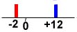
Consider a situation where the North Carolina Tar Heels, for example, score 85 points per game and allow 80 points per game (they've had a rough year). This means that they outscore their opponents by an average of 85-80= 5 ppg. This, however, is just an average; it does not happen in every game. UNC may win by 12 in one game and lose by 2 in the next, giving an average margin of 5 ppg. The Tar Heels won one game and lost the other -- you might say that they were inconsistent. A consistent team would have won both games by 5 points. The Correlated Gaussian method accounts for consistency in the two variance terms, Var(PPG) and Var(PPG allowed). The variance indicates how consistent a team is from game to game. For the Tar Heels, they were not consistently outscoring their opponents, so their variance was relatively high. Pictorally, this is shown below.
This figure shows the distribution of the UNC scoring margin for the two games, with the zero line noted as the separation between games won and games lost. Now imagine how this graph might fill in through the season:
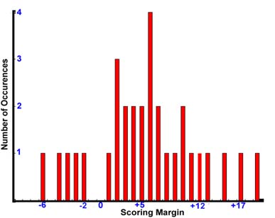
This figure shows the number of games (on the vertical axis) that the difference between UNC and their opponents was what is shown on the horizontal axis. (I'm making these numbers up for the purpose of demonstration.) So the number of times that the difference is greater than zero is the number of times that UNC won and the number of times that the difference is less than zero is the number of times UNC lost.
The important step in arriving at the Correlated Gaussian method is realizing that this plot can be approximated using the well-known statistical Bell Curve, or Gaussian distribution. This distribution has an average of PPG - PPG allowed and a width, as measured by its standard deviation (an average of how much the scoring margin differs from the average scoring margin) of
SQRT[Var(PPG)+Var(PPG Allowed)-2*Cov(PPG,PPG Allowed)]The Correlated Gaussian method is then just a good way of approximating something we know in reality. So why approximate something we know in reality? Because if we have a good approximation that we fully understand, it allows us to better understand the more complex situation we are approximating. In other words, the Correlated Gaussian method simplifies basketball, but does a very good job approximating basketball. By understanding the (relatively) simple Correlated Gaussian method, we better understand the (relatively) complex game.
The power of this method comes from including more information in the variances and in the covariance between the offense and defense. These indicators of consistency are even more important for individuals than for teams. And each of these indicators can be estimated through some statistical theory that I will not go into here. If you have survived this far, you have probably had enough.
The conceptual difficulty for these statistics is then defining scoring possessions, possessions, and points created for individuals. If you read nothing past this sentence (and if you are averse to near-philosophical meanderings through probability theory, you won't), then understand this: individual scoring possessions, possessions, and points created are designed to sum up to the total for the team with credit being assigned to each player according to their (probabilistic) contribution to the score or possession. In other words, I assign individual values of these three statistics so that when you add them up for all players on a team, they equal the team total calculated through other methods. A method that does not do this has an obvious error and I didn't want that.
How credit is assigned is the theoretical challenge, one that I have avoided explaining for years because, as far as I know, it is entirely new to all science and, hence, subject to human error -- the greatest uncertainty of all. The principal is that each player who contributes to his team scoring is credited a fraction of that scoring possession according to the difficulty (or importance) of what they did. If Dennis Scott makes a tough shot off a pass from Penny Hardaway, Scott deserves more credit for the possession than does Hardaway, who made the pass. If our perception of Orlando's chance of scoring was 50% when Hardaway had the ball, but they dropped to 40% when he passed it to Scott in a bad situation, then they went to 100% after Scott hit the shot -- who did the most to help the team? I would say that Scott did. He increased the team's chances from 40% to 100%. Penny actually hurt his team by lowering their chances from 50% to 40%. the net gain for the team was an increase from 50% to 100%, but give Scott +60% and Penny -10%. For this team's one scoring possession, give Scott 60/50 = 1.2 scoring possession and Penny -10/50 = -0.2 scoring possession. The sum of the two is right and I would submit that the credit is attributed properly.
Before you write angrily at that proposal, let me say two things. First, this is an extreme example because usually the assistant (Hardaway) makes a pass that obviously increases the chance of the team scoring, not decreases it, as I demonstrated here. Second, if you don't like the idea, come up with a better one, while still considering the relative lack of data to calculate these things. No one keeps track of the team's probability of scoring within a possession because it is difficult, if not impossible, to measure. We also do not have measurements of how many potential assists are not turned into points, which is important. Point guards do not have statistics reflecting the times they passed to someone who did not make the shot, but the player that did miss the shot does have the negative statistic -- the missed field goal. In my work, this blame is reapportioned. Assistants get credit for their assists, but roughly only 25% of a scoring possession goes to the assistant. The rest goes to the player making the shot. Sometimes, the assistant should get more credit than this -- when they make a tough pass to an open player around the basket -- and rarely should it be as low as in the Scott-Hardaway example. There are some players who generally make good passes for whom this value should be greater. There are also some players who get assists just out of the sheer quantity of passes they make, even if they are not great passes, for whom this value should be lower. The value of 25% has worked pretty well, but it will probably be dynamically estimated in the future.
I said above that all contributors to a scoring possession should get credit. Probabilistically, the biggest contributors are the assistant and the player who made the shot. This is fortunate because we don't have data to get good estimates of the contributions for other players. This is why I emphasize that my methods are approximations, not exact truth. They are good approximations, but there are players for whom they should be questioned.
The individual defensive formulas are much simpler than the individual offensive methods presented above, because methods for defensive evaluation aren't as well developed theoretically. Simply put, I have struggled with evaluating players' defenses for many years now. I came up with a basic method three or four years ago called defensive stops, which are a way of estimating how many times a player stops the opposition from scoring. It's not a bad first approximation, but it misses with players like Joe Dumars and Glenn Rivers, who prevent their assignments from scoring by not allowing them good looks at the basket. They don't get many defensive rebounds or blocks and don't steal the ball much, but they shut down their men. Doug Steele came up with a good way for accounting for this type of player, the kind of player I call a good man defender. On the other hand, my method does best at evaluating team defense, which would include blocks, steals, and defensive rebounds. Doug has begun including these in his method, too, but he uses a form of linear weights, something I disapprove of rather heartily.
Defensive stops occur every time the opposing offense ends a possession without scoring. This can happen via a turnover or a missed shot that the defense rebounds. I evaluate every player on the team as being roughly even in man defense. I do this by finding out how often (times per minute played) the opposition is stopped not through a steal or block, then multiply it by the individual's minutes played. In the formula, this is
Min*[OppFGA-OppFGM-OppOR-TMBLK)/2+(OppTO-TMSTL)]/TMMINThe first part inside the square brackets is how many times the opposition misses a shot, then divided by a factor of two. I divide by two because half of a defensive stop is the missing of the shot -- the other half is getting the defensive rebound. (There is a slight error in logic in the previous statement. See if you can pick up on it.) The second part in the square brackets is the number of turnovers not caused by steals. This is the part that could be aided by using Doug Steele's methodology. It represents an approximation of man defense by assigning everyone on one team the same credit for man defense. Doug matches up each individual player with an opposing assignment and tracks them. This sort of matching is what should eventually replace this part of my formula.
Now we've taken out the individual contributions of blocks, steals, and defensive rebounds to get an average estimate of man defense. It's time to add those back in for each individual. Just adding in an individual's steals and half of both his defensive rebounds and blocks gives an overall formula for defensive stops:
Defensive Stops =
	Min*[OppFGA-OppFGM-OppOR-TMBLK)/2+(OppTO-TMSTL)]/TMMIN
	+ STL + 0.5*(DR+BLK)
Again, remember where we are and where we want to go. We have an offensive rating from above and now we need a defensive rating. We have defensive stops, not a defensive rating. We need to estimate "how many points per possession a player gives up."
This, I'm sorry to say, is difficult to define. How do you evaluate the guard who lets his man drive past him, where his center saves him by blocking the layup attempt? Who gets credit for the stop? Who gets the blame if the layup isn't blocked and goes in? These are theoretical difficulties. Generally, a team plays a style of defense that either asks for help defense or asks for straight man defense or something in between. Depending on whether that guard was supposed to let his man go by determines whether he did something right. If he was supposed to let the man go by, then rotated to the big man's assignment to cut off the dump pass, he apparently did OK. If he was supposed to play straight, then any points scored should mostlly be blamed on him, not the big man covering the little guys' back when it's not his responsibility.
Given this dilemma, how do we proceed? Basically, I try to fit defensive stops into a framework that makes some sense if we ignore the above questions. Ignoring the difficulties sometimes allows one to see a solution. That is my guiding paradigm here.
If we can somehow evaluate how many stops per possession a player has, we essentially have the defensive equivalent of an individual floor percentage. Going from this to a points per possession rating is fairly straightforward. This is the method.
To find the stops per possession, divide a player's total defensive stops by his minutes played, multiply by the team's minutes played, and divide by the team's total number of possessions:
             Stops*TMMIN
Stops/Poss= -------------
             Min*TMPoss.
This number turns out to be very high for some players. For
example, Olajuwon consistently has a stops/poss value of 0.7
or so. This would mean that he stops seven tenths of all
possessions he is responsible for. Or his opponents score
only 30% of the time against him, for a rough rating of
60. Olajuwon is a good defender, but he's not that good.
In order to compensate for this flaw, I weight the team's defensive rating with the individual's stops/poss value. I weight them 80% to 20% because I figure that one player is 20% of his defensive team. It's a little hokey, logically, but it gives results that I'm fairly pleased with, as I mentioned above:
Def. Rtg = 0.8*TMDef.Rtg + 0.2*(200*(1-stops/poss))For completeness, the factor
200*(1-stops/poss)
is an approximation of the points per 100 possessions
arising from the given value of stops/poss.